On the Force Between Two Parallel Plates: A Casimir Calculation, Patiently

A first-principles derivation of the attraction between two perfectly conducting parallel plates, with attention to the regularization scheme and the geometry that motivates it.

Author

Affiliation

R. Cholla

Independent affiliate, Chuck Walla Institute

The geometry, before the equations

Let us consider a region of vacuum bounded by two parallel, perfectly conducting plates of large area \(A\), separated by a distance \(a\) along the \(z\)-axis. The plates are taken to be neutral and grounded; the region between them is empty in the ordinary sense — no matter, no fields, no light. The geometry is the simplest possible: two flat surfaces, parallel, facing one another across a fixed gap.

The classical electromagnetism of this configuration is uneventful. The capacitance is finite; the static fields are zero. The plates do not, in any classical sense, interact.

The quantum electrodynamics of the configuration is not uneventful. The plates impose a boundary condition on the electromagnetic field — the tangential electric field must vanish on each conducting surface — and this boundary condition selects a discrete set of allowed standing-wave modes between them, each of which contributes its zero-point energy \(\frac{1}{2}\hbar \omega\) to the vacuum. The total zero-point energy of the bounded region is therefore different from what it would be in the unbounded vacuum, and the difference is finite once the appropriate cancellations are made. The plates attract.

The result, due to Casimir (1948), is that the force per unit area is

\[ P(a) \;=\; -\,\frac{\pi^{2}}{240}\,\frac{\hbar c}{a^{4}}, \tag{1}\]

attractive, falling off as the inverse fourth power of the separation, and depending on no parameter of the plates other than that they are ideal conductors. The cleanness of the result is the cleanness of the geometry. We shall recover Equation 1 with care.

The mode sum

Between the plates, the electromagnetic field is most cleanly expanded in the modes that satisfy the boundary conditions. For each pair of transverse wavevectors \(\mathbf{k}_{\perp} \in \mathbb{R}^{2}\) and longitudinal mode index \(n = 0, 1, 2, \ldots\), there are two polarizations (with \(n=0\) contributing only one), and the angular frequency of the corresponding mode is

\[ \omega_{n}(\mathbf{k}_{\perp}) \;=\; c\,\sqrt{\,k_{\perp}^{2} + (n\pi/a)^{2}\,}. \tag{2}\]

The zero-point energy per unit plate area, formally, is the sum

\[ \mathcal{E}(a) \;=\; \frac{\hbar}{2} \sum_{n=0}^{\infty}{}^{\!\!\prime}\, \int\!\!\frac{d^{2}k_{\perp}}{(2\pi)^{2}}\; \omega_{n}(\mathbf{k}_{\perp}), \tag{3}\]

with the prime indicating that the \(n=0\) term is to be counted with weight \(\tfrac{1}{2}\), on account of its single polarization.

The sum Equation 3 is, of course, divergent. This is where the Casimir literature begins, and where most introductory accounts pause to apologize. I do not think an apology is in order. The divergence is not a defect of the calculation; it is a feature of the formal vacuum energy, which is unphysical in absolute terms and becomes physical only in differences. The physical quantity is

\[ E_{\text{Cas}}(a) \;=\; \mathcal{E}(a) - \mathcal{E}(\infty), \tag{4}\]

where \(\mathcal{E}(\infty)\) is the same sum performed with the plates removed — that is, with the discrete index \(n\) replaced by a continuous integral. The two divergences cancel, and what remains is finite.

To extract the finite part we regularize, as is conventional, by introducing a smooth cutoff function \(f(\omega/\Lambda)\) which is unity for \(\omega \ll \Lambda\) and falls off rapidly for \(\omega \gg \Lambda\). The choice of \(f\) does not affect the result. One could equally well analytically continue, in the manner of Plunien et al. (1986), using the Riemann zeta function to assign a finite value to the bare sum; the answer is the same. The cancellation is exact, and on first encounter is surprising.

The regularized result

Substituting Equation 2 into Equation 3, performing the angular part of the \(\mathbf{k}_{\perp}\) integral, and writing \(\xi = a k_{\perp}/\pi\), the regularized energy per unit area takes the form

\[ \mathcal{E}_{\Lambda}(a) \;=\; \frac{\hbar c\,\pi^{2}}{4\,a^{3}}\, \sum_{n=0}^{\infty}{}^{\!\!\prime} \int_{0}^{\infty}\!\xi\, d\xi\;\sqrt{\xi^{2} + n^{2}}\; f\!\left(\tfrac{\pi c}{a\Lambda}\sqrt{\xi^{2}+n^{2}}\right). \]

The corresponding integral with continuous \(n\) is the Euler–Maclaurin “smooth” piece, and the difference between the discrete sum and the integral is the finite Casimir energy. The Euler–Maclaurin formula gives

\[ E_{\text{Cas}}(a) \;=\; -\,\frac{\pi^{2}}{720}\,\frac{\hbar c}{a^{3}} \quad\text{per unit area,} \tag{5}\]

independent of \(\Lambda\) in the limit \(\Lambda \to \infty\). The attractive pressure Equation 1 follows as \(P = -\partial E_{\text{Cas}}/\partial a\).

Numerical evaluation

import numpy as np
import matplotlib.pyplot as plt

hbar = 1.055e-34
c = 3.0e8
a = np.logspace(-9, -4, 600)  # plate separation in meters
P = -(np.pi**2 / 240) * hbar * c / a**4   # pressure (Pa), negative = attractive

fig, ax = plt.subplots()
ax.loglog(a*1e6, -P, color="#a0522d", lw=2.0,
          label=r"$|P| = \pi^2 \hbar c / 240 a^4$")

# Reference pressures
ax.axhline(101325, color="#7a8b6f", lw=0.8, ls=":", alpha=0.7)
ax.text(1.2e-3, 1.5e5, "1 atm", color="#4f5e48", fontsize=8.5, fontstyle="italic")
ax.axhline(1.0, color="#7a8b6f", lw=0.8, ls=":", alpha=0.7)
ax.text(1.2e-3, 1.5, "1 Pa", color="#4f5e48", fontsize=8.5, fontstyle="italic")

# Lamoreaux 1997 range
ax.axvspan(0.6, 6.0, color="#d9b382", alpha=0.35,
           label="Lamoreaux 1997 measurement")

# Annotations
for a_val, label in [(1e-2, "1 μm"), (1e-1, "100 nm"), (1e-3, "10 nm")]:
    pass

ax.set_xlabel(r"plate separation $a$ ($\mu$m)")
ax.set_ylabel(r"|Casimir pressure| (Pa)")
ax.set_xlim(1e-3, 1e2)
ax.legend(loc="upper right", framealpha=0.9, fontsize=9)
ax.grid(alpha=0.25, which="both")
ax.set_facecolor("#faf3e3")
fig.patch.set_facecolor("#faf3e3")
for spine in ax.spines.values():
    spine.set_color("#7a3b1f")
plt.tight_layout()
plt.show()

# Specific values
for a_val in [10e-9, 100e-9, 1e-6, 10e-6]:
    P_val = (np.pi**2/240) * hbar * c / a_val**4
    print(f"a = {a_val*1e9:7.1f} nm   |P| = {P_val:.3e} Pa")

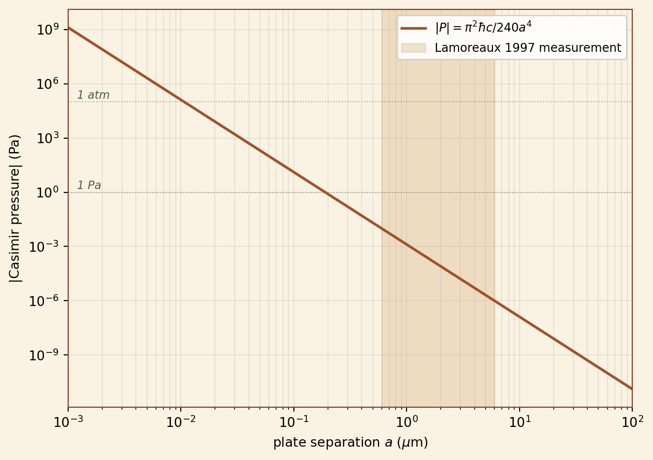
Figure 1: Casimir pressure between two perfectly conducting parallel plates as a function of separation, computed from Equation 1. The shaded region is the regime accessible to the Lamoreaux (1997) measurement (separations from \(0.6\) to \(6\,\mu\text{m}\)); the experimental result agreed with the theoretical prediction at the level of \(5\%\). At a separation of \(10\,\text{nm}\) the pressure approaches one atmosphere.

a =    10.0 nm   |P| = 1.302e+05 Pa
a =   100.0 nm   |P| = 1.302e+01 Pa
a =  1000.0 nm   |P| = 1.302e-03 Pa
a = 10000.0 nm   |P| = 1.302e-07 Pa

The pressure is small at any separation a careful experimentalist would call macroscopic. At \(a = 1\,\mu\text{m}\), \(|P| \approx 1.3\, \text{mPa}\) — about ten thousand times smaller than a millibar of atmospheric pressure. The first credible measurement of Equation 1 in this regime is due to Lamoreaux (1997), who used a torsion pendulum with a spherical lens replacing one of the plates (the sphere-plate geometry being mechanically more tractable, and the geometry having since been treated more carefully than I shall do here, in the proximity-force approximation and beyond). The agreement with theory was within \(5\%\), which is small for this kind of experiment.

At \(a = 10\,\text{nm}\) the pressure is approximately \(10^{5}\, \text{Pa}\), comparable to atmospheric. This is the regime in which the Casimir force becomes structurally relevant in the design of microelectromechanical devices (Chan et al. 2001); it is, in a quite practical sense, what a small enough machine has to push against when it tries to move two of its parts together.

What the geometry has done

I should like to close on the geometry, where I began. The result Equation 1 depends on \(\hbar\), \(c\), and the separation \(a\) — and on nothing else. It does not depend on the material of the plates, provided the plates are good enough conductors at the relevant frequencies. It does not depend on the area \(A\), except trivially through the conversion from energy to pressure. It does not even depend on the choice of regularization. What it depends on is the shape of the boundary: two parallel planes, an infinite gap in transverse coordinates, a finite gap in the third.

A different shape would give a different sign, in some cases. The case of a thin perfectly conducting sphere, treated by Boyer (1968), yields a repulsive self-energy, of magnitude smaller by some four orders of magnitude than the parallel-plate value at the corresponding scale. The cancellations there are more delicate, and the result was, on first encounter in 1968, badly received. It is now, I believe, accepted. Indeed, the geometry will not permit otherwise.

References

Boyer, Timothy H. 1968. “Quantum Electromagnetic Zero-Point Energy of a Conducting Spherical Shell and the Casimir Model for a Charged Particle.” Phys. Rev. 174: 1764–76.

Casimir, H. B. G. 1948. “On the Attraction Between Two Perfectly Conducting Plates.” Proc. K. Ned. Akad. Wet. 51: 793–95.

Chan, H. B., V. A. Aksyuk, R. N. Kleiman, D. J. Bishop, and F. Capasso. 2001. “Quantum Mechanical Actuation of Microelectromechanical Systems by the Casimir Force.” Science 291: 1941–44.

Lamoreaux, S. K. 1997. “Demonstration of the Casimir Force in the 0.6 to 6 \(\mu\)m Range.” Phys. Rev. Lett. 78: 5–8.

Plunien, G., B. Müller, and W. Greiner. 1986. “The Casimir Effect.” Phys. Rep. 134: 87–193.