A Note on the Page–Wootters Construction, with Reference to the Salecker–Wigner Bound

A short technical objection to the proposal that time emerges from the correlation between two clocks: namely, that the clocks themselves cannot be ideal.

Author

Affiliation

M. Yucca

Chuck Walla Institute

Preliminaries

The Director has, in a note from 1986 (Caldera 1986), offered the Page and Wootters (1983) construction as a candidate resolution of the problem of time in canonical quantum gravity. The note is a fine one, and the Page–Wootters mechanism is a fine proposal. The present remark is not directed at the proposal in general but at one technical detail which the Director’s exposition deferred and which, I think, deserves to be stated explicitly. Namely: the clock in a Page–Wootters universe cannot be a physical system in any of the senses that the word ordinarily admits.

The objection has two parts, both classical, both dating from before the proposal itself.

Part one: Pauli’s theorem

The Page–Wootters construction requires a clock subsystem \(B\) whose Hamiltonian \(\hat H_B\) admits a self-adjoint canonical conjugate operator \(\hat T_B\) with continuous spectrum running over all of \(\mathbb{R}\). The conditional state is then defined, as in equation (3) of Caldera (1986), as the projection of the joint state onto an eigenstate of \(\hat T_B\).

Pauli (1933) showed, in a footnote that has been more cited than read, that no such operator can exist if \(\hat H_B\) is bounded below. The argument is short. Suppose \([\hat T_B, \hat H_B] = i\hbar\). Then for any energy eigenstate \(|E\rangle\) and any real \(\epsilon\),

\[ \hat H_B \, e^{-i\epsilon \hat T_B / \hbar} |E\rangle \;=\; (E - \epsilon)\, e^{-i\epsilon \hat T_B / \hbar}|E\rangle, \tag{1}\]

so the spectrum of \(\hat H_B\) contains \(E - \epsilon\) for every real \(\epsilon\), contradicting any lower bound. A self-adjoint \(\hat T_B\) therefore requires a Hamiltonian unbounded below; no physical clock has this.

The remedies are known. One may replace the projection-valued measure of \(\hat T_B\) with a positive operator-valued measure (POVM); one may extend the Hilbert space to admit “covariant” time observables; one may interpret the construction in the sense of Rovelli (1991) as a relational specification of partial observables. Each of these remedies is technical and each modifies the conditional probability in ways that the Director’s exposition would not have admitted without footnoting. The mechanism, in its naive formulation, is therefore an idealization.

Part two: The Salecker–Wigner bound

Setting Pauli aside, suppose one grants the existence of a workable clock observable. There remains a quantitative limit on the precision with which any physically realizable clock — meaning: any system of finite mass and finite energy — can resolve a time interval. The limit was derived by Salecker and Wigner (1958) and refined by Wigner (1957). It states that a clock of total mass \(M\) which is to operate, as a clock, for a total elapsed time \(T\), has a minimum resolvable time interval

\[ \Delta t \;\geq\; \sqrt{\frac{\hbar T}{M c^{2}}}. \tag{2}\]

The result follows from elementary uncertainty arguments: a clock of energy uncertainty \(\Delta E\) has a time resolution \(\Delta t \sim \hbar/\Delta E\); over a total operating time \(T\) the wavefunction of a clock of mass \(M\) spreads spatially by at least \(\sqrt{\hbar T / M}\); combining these, with \(\Delta E \leq Mc^{2}\), yields Equation 2.

The bound is not a function of the clock’s design. It is a consequence of quantum mechanics together with the finiteness of the clock’s mass.

Numerical evaluation

Let us substitute the numbers, as is the habit of the house.

import numpy as np
import matplotlib.pyplot as plt

hbar = 1.055e-34
c = 3.0e8
T = 365.25 * 24 * 3600   # 1 year, in seconds

M = np.logspace(-30, 5, 600)   # mass in kg, from atomic to a small house
dt_min = np.sqrt(hbar * T / (M * c**2))

fig, ax = plt.subplots()
ax.loglog(M, dt_min, color="#2b2118", lw=2.0)

events = [
    ("electron",                    9.11e-31, "#7a8b6f"),
    ("Cs-133 atom",                 2.21e-25, "#7a8b6f"),
    ("a brass railroad clock",      2.0,      "#a0522d"),
    ("the Director's pickup truck", 2.0e3,    "#7a3b1f"),
    ("Planck mass",                 2.18e-8,  "#b8794f"),
]

for label, M_val, color in events:
    dt_val = np.sqrt(hbar * T / (M_val * c**2))
    ax.plot(M_val, dt_val, "o", color=color, markersize=6, zorder=5)
    ax.annotate(label, xy=(M_val, dt_val),
                xytext=(M_val*1.7, dt_val*0.25),
                fontsize=8.5, color=color, fontstyle="italic")

# Reference: Cs-133 atomic clock published precision ~1e-15 s
ax.axhline(1e-15, color="#4f5e48", lw=0.8, ls=":", alpha=0.7)
ax.text(1e-30, 3e-15, "Cs-133 clock published $\\Delta t$",
        fontsize=8.5, color="#4f5e48", fontstyle="italic")

ax.set_xlabel(r"clock mass $M$ (kg)")
ax.set_ylabel(r"minimum $\Delta t$ over $T = 1$ yr  (s)")
ax.grid(alpha=0.25, which="both")
ax.set_facecolor("#faf3e3")
fig.patch.set_facecolor("#faf3e3")
for spine in ax.spines.values():
    spine.set_color("#7a3b1f")
plt.tight_layout()
plt.show()

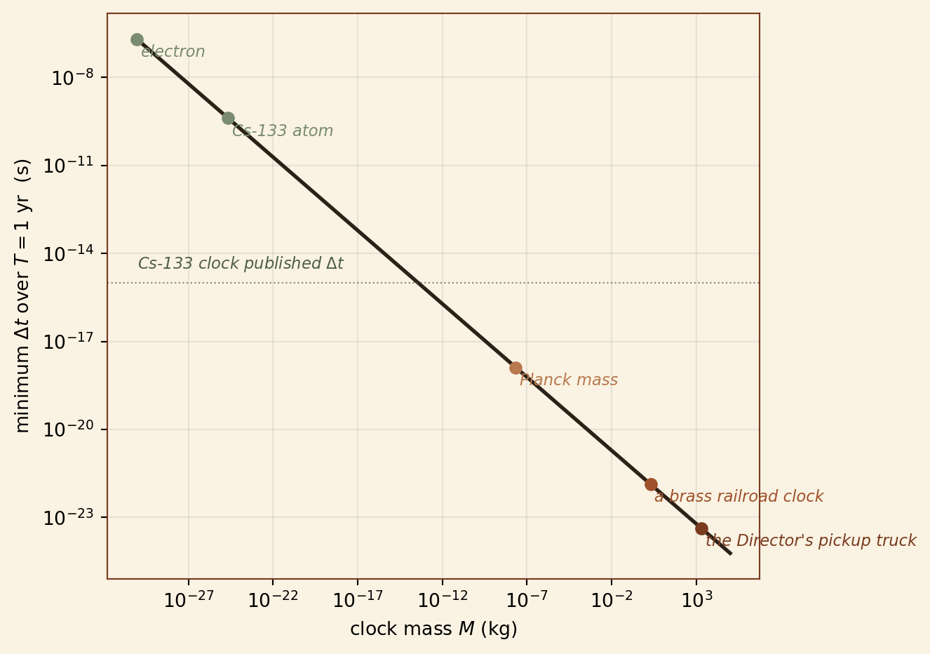
Figure 1: Salecker–Wigner minimum time uncertainty as a function of clock mass, for total elapsed time \(T = 1\,\text{yr}\). The brass railroad clock in the Institute’s seminar room is shown for scale. The Page–Wootters mechanism, as ordinarily presented, takes the limit \(\Delta t \to 0\), which Equation 2 forbids for any finite \(M\).

For the brass railroad clock the bound is \(\Delta t \gtrsim 10^{-22}\,\text{s}\), which is far below the resolution of the hands and below any timescale of seminar interest. For an atomic clock the bound is approximately \(10^{-13}\,\text{s}\), which is within an order of magnitude of the published precision of caesium references and is the source of the long-running interest in heavier-atom standards.

The bound is not in conflict with any practical use of clocks. It is, however, in conflict with the idealization that the clock \(B\) in a Page–Wootters universe can be made arbitrarily precise without also being made arbitrarily massive. Indeed, by the time the clock has acquired enough mass to track time at any chosen precision over cosmological intervals, it has acquired enough mass to disturb, gravitationally, the system \(A\) which it is supposed to be correlated with but not to perturb (Hartle 1988).

A short conclusion

The Page–Wootters mechanism is a useful and probably correct picture of how time emerges in a closed quantum universe. It is not a mechanism that operates without cost. The cost is paid in the physical clock — in its mass, its precision, and its gravitational coupling — and the cost has been carefully bounded by classical results (Pauli (1933), Salecker and Wigner (1958), Wigner (1957)) which the proposal does not modify.

I make this remark not to disagree with the Director, with whom I agree on the essentials, but because at the Institute we have made something of a habit, when proposing that an apparent difficulty has been resolved, of asking what the resolution costs. The answer here is small and bounded, but it is not zero.

References

Caldera, D. R. 1986. “The Wheeler–DeWitt Equation and the Disappearance of \(t\).” Notes & Preprints, Chuck Walla Institute.

Hartle, James B. 1988. “Quantum Mechanics of Cosmological Observations.” Phys. Rev. D 37: 2818–32.

Page, Don N., and William K. Wootters. 1983. “Evolution Without Evolution: Dynamics Described by Stationary Observables.” Phys. Rev. D 27: 2885–92.

Pauli, Wolfgang. 1933. “Die allgemeinen Prinzipien der Wellenmechanik.” Handbuch Der Physik 24: 83–272.

Rovelli, Carlo. 1991. “Time in Quantum Gravity: An Hypothesis.” Phys. Rev. D 43: 442–56.

Salecker, H., and E. P. Wigner. 1958. “Quantum Limitations of the Measurement of Space-Time Distances.” Phys. Rev. 109: 571–77.

Wigner, E. P. 1957. “Relativistic Invariance and Quantum Phenomena.” Rev. Mod. Phys. 29: 255–68.