The Cosmological Constant: A Casimir Reading of the Cohen–Kaplan–Nelson Bound

On a recent and somewhat overlooked argument that the gravitating vacuum energy in a region of finite size is bounded by a quantity which, for the cosmological horizon, is approximately the observed value; and on what the geometry of the boundary may have to do with the sign of the result.

Author

Affiliation

R. Cholla

Independent affiliate, Chuck Walla Institute

Preliminary

The cosmological constant problem, in the form Weinberg (1989) set out, is the discrepancy of approximately \(10^{120}\) between the naïve quantum-field-theoretic estimate of the vacuum energy density and the value observed in the late-time acceleration of the universe. The discrepancy is, by some margin, the largest in contemporary physics. The literature is vast and the reviews are many (Padmanabhan 2003; Polchinski 2006); I shall not undertake to survey it.

I wish, in this note, to consider one particular argument — due to Cohen et al. (1999), and pursued by various authors since (Hsu 2004; Banks and Fischler 2004) — which has the property of relating two quantities that have, on the standard formulation of the problem, no business being related. The argument observes that an effective field theory in a finite region, with both a UV cutoff \(\Lambda\) and an IR cutoff \(L\), is constrained by the requirement that the field-theory states it describes do not, by their own gravitating mass, collapse the region into a black hole. This requirement, when applied to the case in which \(L\) is the cosmological horizon, yields a bound on the gravitating vacuum energy density which is, numerically and perhaps to within order unity, the observed value of \(\rho_{\Lambda}\).

The result is striking. It is also, I think, susceptible of a reading that has not been fully drawn out in the literature, and which is naturally suggested by the geometry of the Casimir effect. The reading concerns the sign of the result, to which I shall return in §4.

§1 — The Cohen–Kaplan–Nelson argument

The argument is short and I shall reproduce it. Consider an effective field theory defined in a region of size \(L\), valid up to some UV cutoff \(\Lambda \ll L^{-1}\). The vacuum energy density contributed by modes between zero momentum and the cutoff is, on dimensional grounds,

\[ \rho_{\text{vac}} \;\sim\; \Lambda^{4}, \]

and the total vacuum energy contained in the region is

\[ E_{\text{vac}} \;\sim\; \Lambda^{4} L^{3}. \]

The Schwarzschild radius corresponding to the energy \(E_{\text{vac}}\) is \(r_{S} \sim G E_{\text{vac}} \sim L^{3}\Lambda^{4}/M_{P}^{2}\), where \(M_{P} = G^{-1/2}\) is the (non-reduced) Planck mass. The requirement that the region not be inside its own Schwarzschild radius — that is, \(r_{S} \lesssim L\) — yields

\[ \Lambda^{4} \;\lesssim\; \frac{M_{P}^{2}}{L^{2}}. \tag{1}\]

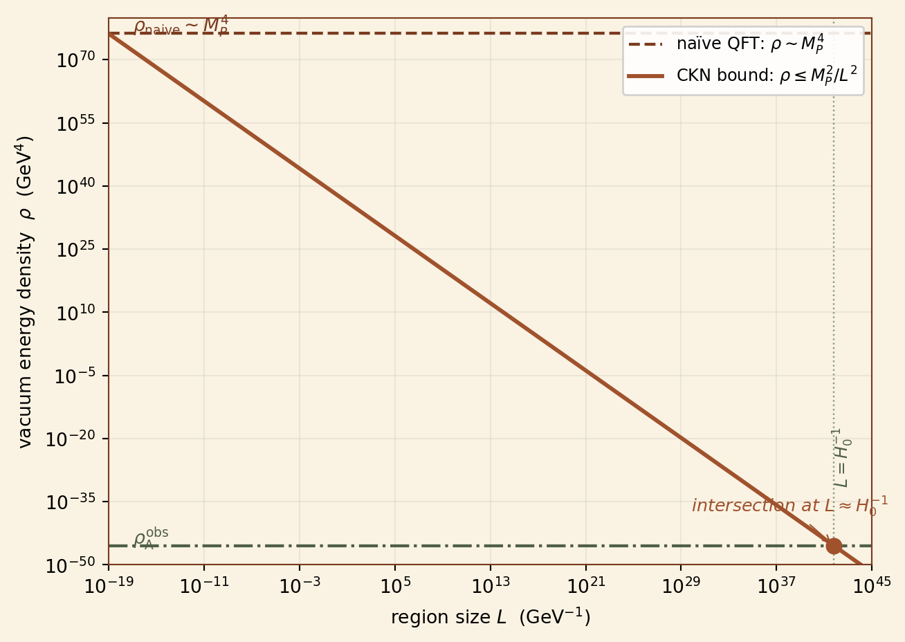
This is the Cohen–Kaplan–Nelson bound. The vacuum energy density in a region of size \(L\) is, accordingly, bounded by

\[ \rho_{\text{vac}} \;\lesssim\; \frac{M_{P}^{2}}{L^{2}}. \tag{2}\]

The bound is geometric. It depends on \(L\), the size of the region; it does not depend on \(\Lambda\) except through the constraint Equation 1, which relates \(\Lambda\) to \(L\).

Setting \(L\) equal to the cosmological horizon, \(L \sim H_{0}^{-1}\), the bound becomes

\[ \rho_{\text{vac}} \;\lesssim\; M_{P}^{2}\, H_{0}^{2}, \tag{3}\]

a quantity that is, to within a small numerical factor, the observed value of the cosmological constant. The naïve QFT estimate \(\rho_{\text{vac}} \sim M_{P}^{4}\) overshoots this by a factor of \((M_{P}/H_{0})^{2} \approx 10^{120}\), which is, recognizably, the discrepancy of Weinberg (1989).

§2 — A figure

import numpy as np
import matplotlib.pyplot as plt

# Natural units: GeV
M_P = 1.22e19              # Planck mass (non-reduced), GeV
H0  = 1.5e-42              # H_0 in GeV
rho_obs = M_P**2 * H0**2   # ~ observed Lambda density, GeV^4
rho_naive = M_P**4

# L in GeV^-1
L_horizon = 1.0 / H0
L = np.logspace(np.log10(1e-19), np.log10(1e45), 600)

# CKN bound: rho ≤ M_P^2 / L^2
rho_CKN = M_P**2 / L**2

fig, ax = plt.subplots()

# Naive estimate
ax.axhline(rho_naive, color="#7a3b1f", lw=1.6, ls="--",
           label=r"naïve QFT: $\rho \sim M_P^4$")
ax.text(1e-17, rho_naive*3, r"$\rho_\mathrm{naive} \sim M_P^4$",
        color="#7a3b1f", fontsize=10, fontstyle="italic")

# CKN bound
ax.loglog(L, rho_CKN, color="#a0522d", lw=2.2,
          label=r"CKN bound: $\rho \leq M_P^2 / L^2$")

# Observed
ax.axhline(rho_obs, color="#4f5e48", lw=1.6, ls="-.")
ax.text(1e-17, rho_obs*3, r"$\rho_\Lambda^\mathrm{obs}$",
        color="#4f5e48", fontsize=10, fontstyle="italic")

# Mark Hubble scale
ax.axvline(L_horizon, color="#7a8b6f", lw=0.9, ls=":", alpha=0.85)
ax.text(L_horizon*0.6, 1e-30, r"$L = H_0^{-1}$",
        color="#4f5e48", fontsize=9, fontstyle="italic", rotation=90)

# Mark intersection of CKN with observed
L_intersect = M_P / np.sqrt(rho_obs)
ax.plot(L_intersect, rho_obs, "o", color="#a0522d", markersize=8, zorder=5)
ax.annotate("intersection at $L \\approx H_0^{-1}$",
            xy=(L_intersect, rho_obs),
            xytext=(L_intersect*1e-12, rho_obs*1e8),
            fontsize=9.5, color="#a0522d", fontstyle="italic",
            arrowprops=dict(arrowstyle="->", color="#a0522d", lw=0.8))

ax.set_xlabel(r"region size $L$  (GeV$^{-1}$)")
ax.set_ylabel(r"vacuum energy density  $\rho$  (GeV$^4$)")
ax.set_xlim(1e-19, 1e45)
ax.set_ylim(1e-50, 1e80)
ax.legend(loc="upper right", framealpha=0.9, fontsize=9)
ax.grid(alpha=0.2, which="both")
ax.set_facecolor("#faf3e3")
fig.patch.set_facecolor("#faf3e3")
for spine in ax.spines.values():
    spine.set_color("#7a3b1f")
plt.tight_layout()
plt.show()

# Print the intersection
print(f"Hubble length L = 1/H_0      ≈ {L_horizon:.2e} GeV^-1")
print(f"CKN-observed crossing scale  ≈ {L_intersect:.2e} GeV^-1")
print(f"ratio                         = {L_intersect/L_horizon:.3f}")

Figure 1: Vacuum energy density as a function of the size \(L\) of the region in which an effective field theory is consistently defined. The naïve QFT estimate \(\rho \sim M_{P}^{4}\) is the upper horizontal line. The Cohen–Kaplan–Nelson bound \(\rho \leq M_{P}^{2}/L^{2}\) is the descending diagonal. The observed cosmological-constant density \(\rho_{\Lambda,\text{obs}}\) is the lower horizontal line. The intersection of the diagonal with the observed value occurs at \(L \sim H_{0}^{-1}\), the size of the cosmological horizon.

Hubble length L = 1/H_0      ≈ 6.67e+41 GeV^-1
CKN-observed crossing scale  ≈ 6.67e+41 GeV^-1
ratio                         = 1.000

The crossing of the diagonal with the observed value occurs at the scale of the visible universe to within a factor of order unity. This is, on first encounter, a remarkable coincidence. It is the content of the CKN argument.

§3 — What the bound is, and is not

Let us be careful about what Equation 2 establishes and what it does not.

It establishes that the vacuum energy density of an effective field theory consistently defined in a region of size \(L\) is at most of order \(M_{P}^{2}/L^{2}\). It does not establish that the vacuum energy density is of this order. The bound is an upper bound; it becomes saturated only in regimes where the field theory is, in some sense, maximally populated. There is no general reason, in the present formulation, why a typical patch of vacuum should saturate the bound, and the literature has not — to my knowledge — produced a derivation of saturation from first principles.

What the argument does establish, and what is, I think, its real content, is the following: the discrepancy of \(10^{120}\) between the naïve estimate and the observed value is, in part, an artifact of applying the naïve estimate in a regime where it is not valid. If the IR cutoff is the cosmological horizon, then the UV cutoff \(\Lambda\) of the gravitating vacuum modes is bounded above by approximately \(10^{-3}\,\text{eV}\), not by the Planck mass. The vacuum modes between \(10^{-3}\,\text{eV}\) and \(M_{P}\) are not absent from the field theory; they are, however, modes whose contribution to gravitating vacuum energy is, by the consistency of the theory, bounded by Equation 1.

The argument therefore does not solve the cosmological constant problem. It rephrases it. The new question — and it is, I believe, a sharper question than the old one — is why the IR cutoff should be the cosmological horizon, and why the bound Equation 3 should be saturated rather than merely respected.

To these questions I have no answer, and the literature has none either; the proposals of Banks and Fischler (2004) and Hsu (2004) are intriguing but not, I think, conclusive. I do not undertake to settle the matter in the present note.

§4 — On the sign

The CKN bound is, as stated in Equation 3, a bound on \(|\rho_{\text{vac}}|\). It does not, on its face, fix the sign of the result. The observed cosmological constant is positive. Why positive, rather than negative — or zero?

I wish, here, to make a remark which is not, strictly speaking, a derivation, but which seems to me suggestive.

The Casimir effect is the physically measurable consequence of mode redistribution under boundary conditions. For two parallel plates the Casimir energy per unit area is \(-\pi^{2}\hbar c/720 a^{3}\) (Casimir 1948), and the resulting force is attractive. For a thin perfectly conducting spherical shell, by contrast, the self-energy is positive (Boyer 1968), by an amount approximately \(+0.046\,\hbar c/R\). The two cases are derived from the same formalism. The sign difference arises entirely from the geometry of the boundary.

The cosmological constant problem, on the CKN reading, is a problem about the vacuum energy of a finite region with an IR cutoff. The IR cutoff is, in the cosmological context, a horizon; and a horizon, viewed instantaneously, has the topology of a sphere. The analogy with Boyer’s case is not perfect — the cosmological horizon is not a perfect conducting shell, the modes of the gravitating vacuum are not the modes of the photon field, and the regularization scheme is not the same — but the structural feature responsible for the sign in the Casimir case is the same structural feature one would expect to be operative here: namely, that the vacuum energy of a region bounded by a closed, positively-curved surface is, on geometric grounds, a different quantity, and possibly of a different sign, than the vacuum energy of a region bounded by parallel planes.

If this analogy is to be trusted — and I am not at all certain that it should be trusted to within a factor of order unity, much less to better — then the positivity of the observed cosmological constant may be, in part, a topological consequence of the de Sitter horizon’s being a sphere. The cosmological constant is positive because the universe, in its de Sitter phase, is bounded, in the relevant sense, by a sphere; if it were bounded by parallel planes, it would not be.

I do not advance this as a proof. I advance it as an observation: that the same mathematics which predicts that two plates attract and a sphere repels would, applied with the appropriate care and with attention to the differences between the cases, predict the sign of the cosmological constant. The sign of a result, in Casimir physics, is rarely accidental. Indeed, the geometry will not permit otherwise.

§5 — What survives

I have argued, in outline, the following. The Cohen–Kaplan–Nelson bound Equation 2 is a real and surprising relation between the size of a region and the gravitating vacuum energy it can contain. It does not solve the cosmological constant problem; it sharpens the question to: why is the IR cutoff the cosmological horizon, and why is the bound saturated? The geometric structure of the bound is, I think, consonant with a Casimir-style reading, and the sign of the cosmological constant — its positivity — may be a consequence of the topological character of the de Sitter horizon, in approximately the same sense that the sign of Boyer’s result is a consequence of the spherical character of the conducting shell.

What survives, then, is not a solution but a reorientation. The quantity to be explained is no longer \(10^{-122}\, M_{P}^{4}\), a number that has no internal structure and resists any natural account. It is, rather, a number that has the form \(M_{P}^{2}/L^{2}\), in which \(L\) is the cosmological horizon — a quantity that does, on the geometric reading, have an internal structure, and one whose account is now reduced to two more tractable subordinate questions. Whether those questions have natural answers is for those better qualified than I to pursue. The matter is not settled; the matter, on this reading, is at least posed.

References

Banks, T., and W. Fischler. 2004. “An Holographic Cosmology.” arXiv:hep-Th/0405200.

Boyer, Timothy H. 1968. “Quantum Electromagnetic Zero-Point Energy of a Conducting Spherical Shell and the Casimir Model for a Charged Particle.” Phys. Rev. 174: 1764–76.

Casimir, H. B. G. 1948. “On the Attraction Between Two Perfectly Conducting Plates.” Proc. K. Ned. Akad. Wet. 51: 793–95.

Cohen, Andrew G., David B. Kaplan, and Ann E. Nelson. 1999. “Effective Field Theory, Black Holes, and the Cosmological Constant.” Phys. Rev. Lett. 82: 4971–74.

Hsu, Stephen D. H. 2004. “Entropy Bounds and Dark Energy.” Phys. Lett. B 594: 13–16.

Padmanabhan, T. 2003. “Cosmological Constant — the Weight of the Vacuum.” Phys. Rep. 380: 235–320.

Polchinski, Joseph. 2006. “The Cosmological Constant and the String Landscape.” arXiv:hep-Th/0603249.

Weinberg, Steven. 1989. “The Cosmological Constant Problem.” Rev. Mod. Phys. 61: 1–23.