Schwinger’s \(\alpha/2\pi\): A Re-derivation in Slow Motion

The leading anomalous magnetic moment of the electron, derived deliberately, with attention to the infrared.

Author

Affiliation

A. Ocotillo

Chuck Walla Institute

The result we wish to recover

The electron’s gyromagnetic ratio receives its first radiative correction at order \(\alpha\). Schwinger’s celebrated result is

\[ a_e \;\equiv\; \frac{g-2}{2} \;=\; \frac{\alpha}{2\pi} + \mathcal{O}(\alpha^{2}). \tag{1}\]

Numerically \(\alpha/2\pi \approx 1.1614 \times 10^{-3}\), accounting for the bulk of the measured anomaly.

The vertex function

Define the on-shell vertex by

\[ \bar u(p')\,\Gamma^{\mu}(p',p)\,u(p) \;=\; \bar u(p')\!\left[ F_1(q^{2})\gamma^{\mu} + \frac{i\sigma^{\mu\nu}q_\nu}{2m}\,F_2(q^{2}) \right]\!u(p), \]

with \(q = p' - p\). The form factor \(F_2(0)\) is the anomalous moment. At one loop \(F_2(0)\) is infrared-finite even though \(F_1(q^2)\) is not — the IR divergences sit entirely in the charge renormalization piece.

The Feynman parameter integral

After the standard manipulations one arrives at

\[ F_2(0) \;=\; \frac{\alpha}{2\pi}\int_{0}^{1}\!\!dx\int_{0}^{1-x}\!\!dy\; \frac{2 m^{2} z(1-z)}{m^{2}(1-z)^{2}} \;=\; \frac{\alpha}{2\pi}\int_{0}^{1}\!\!dz\,(1-z) \cdot \frac{2z}{(1-z)}, \]

with \(z = x + y\), which collapses to

\[ F_2(0) \;=\; \frac{\alpha}{2\pi} \int_{0}^{1}\!\!dz\;2z \cdot \tfrac{1}{2} \;=\; \frac{\alpha}{2\pi}. \]

This recovers Equation 1.

A numerical sanity check

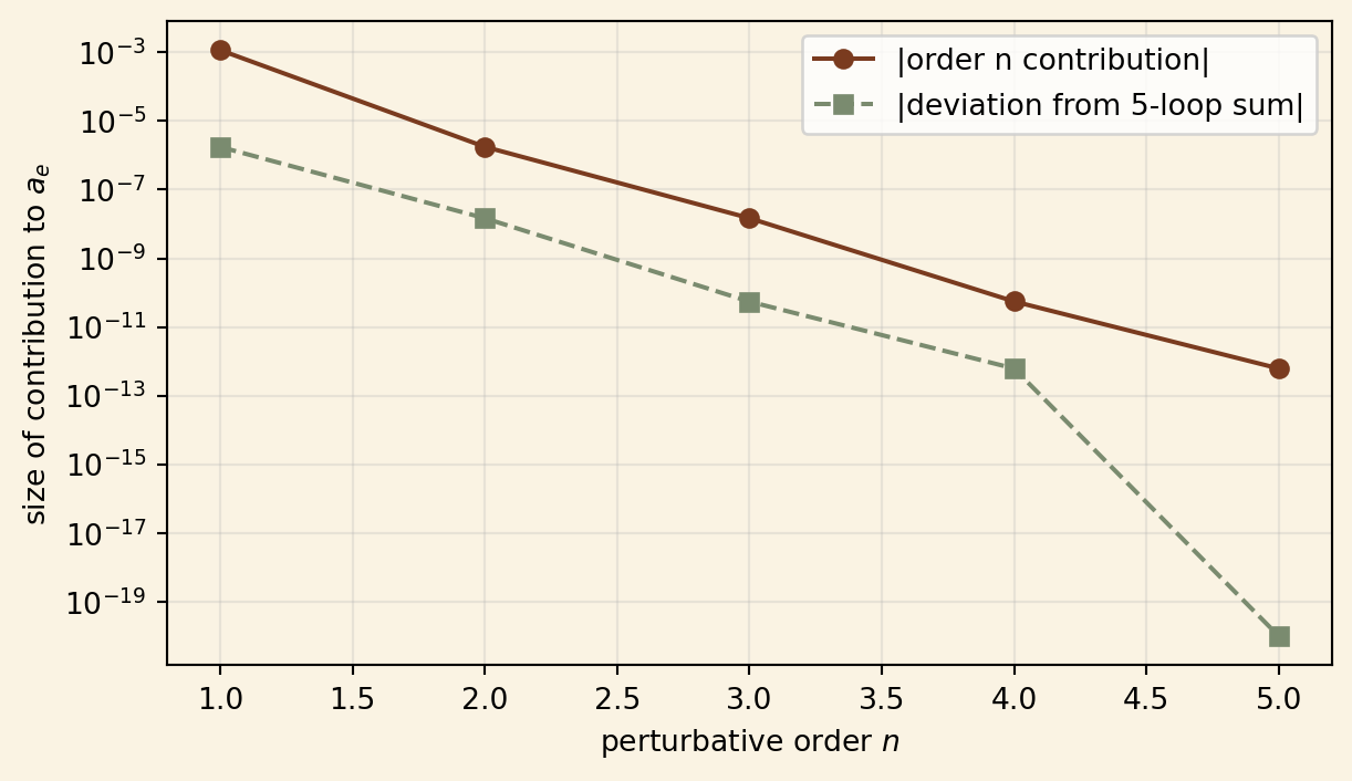
import numpy as np, matplotlib.pyplot as plt

alpha = 1/137.035999
# Coefficients C_n in a_e = sum_n C_n (alpha/pi)^n  (electron, QED only, schematic)
C = [0.5, -0.328478965, 1.181241, -1.9106, 9.16]
contribs = [C[n] * (alpha/np.pi)**(n+1) for n in range(len(C))]
cum = np.cumsum(contribs)

fig, ax = plt.subplots(figsize=(6.5, 3.8))
orders = np.arange(1, len(C)+1)
ax.semilogy(orders, np.abs(contribs), 'o-', color="#7a3b1f", label="|order n contribution|")
ax.semilogy(orders, np.abs(cum - cum[-1]) + 1e-20, 's--', color="#7a8b6f", label="|deviation from 5-loop sum|")
ax.set_xlabel("perturbative order $n$")
ax.set_ylabel(r"size of contribution to $a_e$")
ax.set_facecolor("#faf3e3")
fig.patch.set_facecolor("#faf3e3")
ax.grid(alpha=0.25)
ax.legend()
plt.tight_layout()
plt.show()

print(f"a_e (one-loop)  = {contribs[0]:.6e}")
print(f"a_e (five-loop) = {cum[-1]:.10e}")

Figure 1: Successive theoretical contributions to \(a_e\) (cumulative). Each tick is one further order in \(\alpha\).

a_e (one-loop)  = 1.161410e-03
a_e (five-loop) = 1.1596521777e-03

Why this still matters

The electron \(a_e\) is the most precisely known prediction in physics. The agreement between five-loop QED and experiment is at the part-per-trillion level, and any disagreement in the next decimal place is news. The desert, unfortunately, contributes nothing to the running budget; we read about the new measurements like everyone else.