A Note on the Running of the QED Coupling

One-loop \(\beta\)-function, the Landau pole, and a plot of \(\alpha(\mu)\) from the electron mass to the TeV scale.

Author

Affiliation

M. Yucca

Chuck Walla Institute

Setting

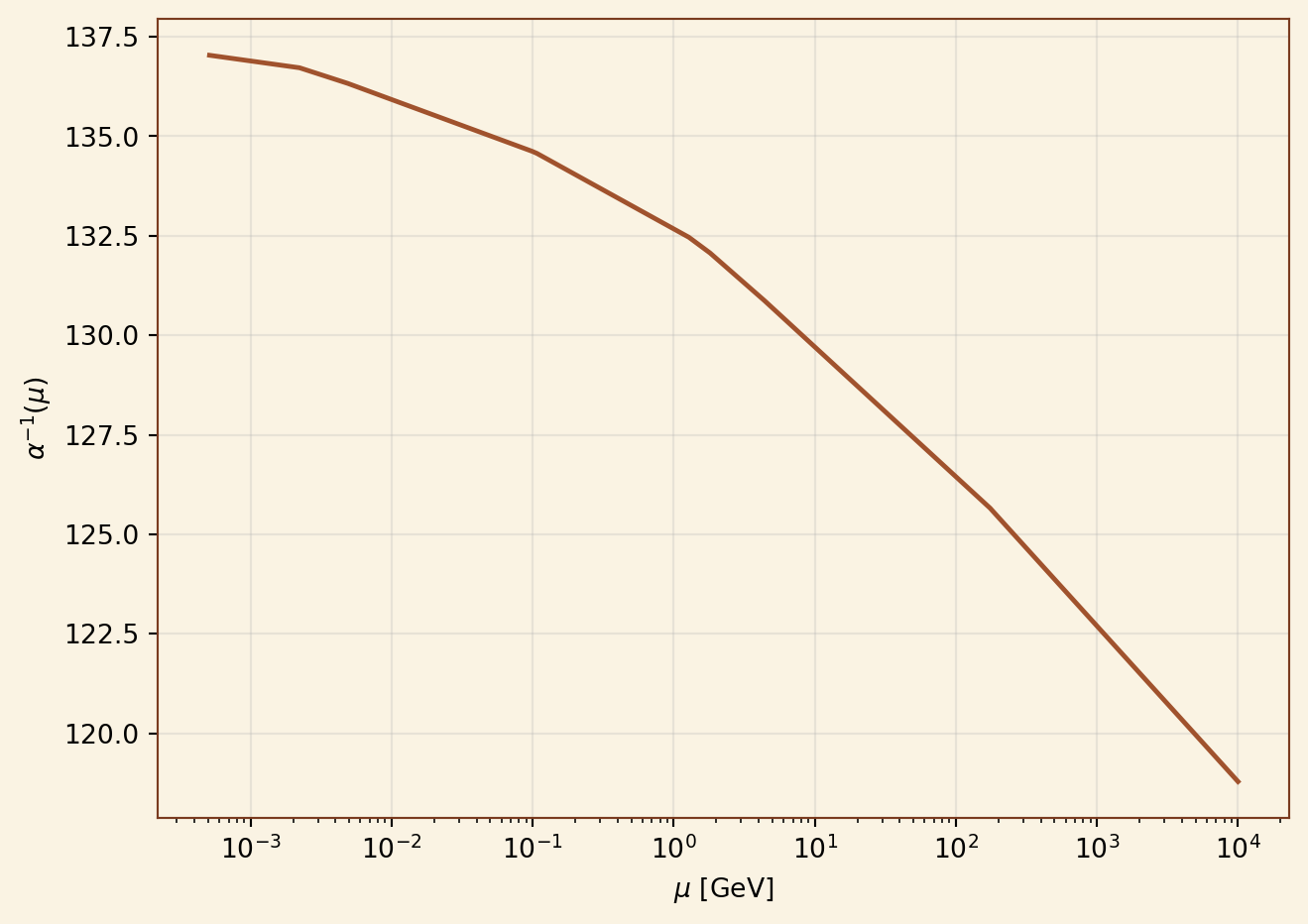
The fine-structure constant is famously not constant. In QED, the renormalized coupling \(\alpha(\mu)\) depends on the energy scale \(\mu\) at which it is probed. At low energies one measures \(\alpha^{-1}(m_e) \approx 137.036\); at the \(Z\)-pole, \(\alpha^{-1}(M_Z) \approx 127.9\) (Peskin and Schroeder 1995).

This note records the one-loop derivation, plots \(\alpha(\mu)\) across fifteen decades, and remarks on the Landau pole.

The one-loop \(\beta\)-function

The QED \(\beta\)-function at one loop, in the on-shell scheme with a single charged fermion of charge \(Q_f\), is

\[ \beta(\alpha) \;=\; \mu \frac{\partial \alpha}{\partial \mu} \;=\; \frac{2\alpha^{2}}{3\pi}\sum_{f} Q_f^{2}\,\Theta(\mu - m_f), \tag{1}\]

where the step function counts only fermions lighter than the probe scale. Solving Equation 1 with the boundary condition \(\alpha(\mu_0) = \alpha_0\) gives

\[ \alpha(\mu) \;=\; \frac{\alpha_0}{1 - \dfrac{2\alpha_0}{3\pi}\sum_{f} Q_f^{2} \log(\mu/\mu_0)}. \tag{2}\]

Two features deserve comment:

• The denominator vanishes at the Landau pole \(\mu_{\text{LP}} = \mu_0 \exp\!\left[\frac{3\pi}{2\alpha_0 \sum Q_f^{2}}\right]\), located at an absurdly high energy and not believed to be physical.
• New charged species speed up the running once \(\mu\) exceeds their masses, visible as kinks in Figure 1.

Numerical evaluation

We integrate Equation 2 across the Standard Model charged fermion spectrum.

import numpy as np
import matplotlib.pyplot as plt

# Charged-fermion masses (GeV) and charges
fermions = [
    ("e",   0.000511,  -1),
    ("mu",  0.1057,    -1),
    ("u",   0.0022,    +2/3),
    ("d",   0.0047,    -1/3),
    ("s",   0.095,     -1/3),
    ("tau", 1.777,     -1),
    ("c",   1.27,      +2/3),
    ("b",   4.18,      -1/3),
    ("t",   172.7,     +2/3),
]
# Color factor for quarks
def Nc(name): return 3 if name in {"u","d","s","c","b","t"} else 1

alpha0_inv = 137.036
mu0 = 0.000511  # m_e in GeV

mus = np.logspace(np.log10(mu0), np.log10(1e4), 4000)

def alpha_inv(mu):
    s = 0.0
    for name, m, Q in fermions:
        if mu > m:
            s += Nc(name) * Q**2 * np.log(mu / m)
    return alpha0_inv - (2/(3*np.pi)) * s

vals = np.array([alpha_inv(m) for m in mus])

fig, ax = plt.subplots()
ax.plot(mus, vals, color="#a0522d", lw=1.8)
ax.set_xscale("log")
ax.set_xlabel(r"$\mu$ [GeV]")
ax.set_ylabel(r"$\alpha^{-1}(\mu)$")
ax.grid(alpha=0.25)
ax.set_facecolor("#faf3e3")
fig.patch.set_facecolor("#faf3e3")
for spine in ax.spines.values():
    spine.set_color("#7a3b1f")
plt.tight_layout()
plt.show()

Figure 1: One-loop running of \(\alpha^{-1}(\mu)\) from \(m_e\) to \(10\,\text{TeV}\). Kinks at each charged-fermion threshold.

At \(\mu = M_Z \approx 91.19\,\text{GeV}\) the one-loop estimate gives

alpha^-1(M_Z) ≈ 126.58  (one-loop, leptons + quarks)

which lands within a percent of the precise value, the residual gap being absorbed by two-loop corrections and hadronic threshold effects.

A short table of milestones

Scale \(\mu\)	\(\alpha^{-1}(\mu)\) (one-loop)
\(m_e = 0.511\,\text{MeV}\)	\(137.04\)
\(m_\tau = 1.78\,\text{GeV}\)	\(\approx 133.5\)
\(M_Z = 91.2\,\text{GeV}\)	see above
\(10\,\text{TeV}\)	see plot

Remarks

The one-loop running already captures the essential phenomenon — the coupling strengthens as we probe shorter distances — and the formula Equation 2 is useful precisely because it is wrong in interesting ways. The triviality of QED is then not a defect of the calculation but a hint that QED, taken as a fundamental theory, must be embedded in a larger structure.

References

Peskin, Michael E., and Daniel V. Schroeder. 1995. An Introduction to Quantum Field Theory. Addison-Wesley.