The Calico Tanks Barrier, Re-examined: A Transfer-Matrix Sequel

We revisit the WKB calculation of Ocotillo (2011) with a transfer-matrix method, vindicating M. Yucca’s correction and recovering an exact transmission coefficient that differs from the WKB estimate by a factor of two.

Authors

Affiliations

A. Ocotillo

Chuck Walla Institute

J. Saguaro

Sonoran Polytechnic; visiting

A correction owed

The May 2011 note (Ocotillo 2011) computed, by way of an introductory exercise, the WKB transmission coefficient through a one-dimensional potential barrier whose profile was lifted from a sandstone crest in the Calico Hills of Red Rock Canyon. The result, \(T_{\text{WKB}} \approx 10^{-7}\), was reported with an explicit caveat: M. Yucca, in a brief note appended to that post, had observed that the profile contains a feature on the leeward face whose curvature in scaled coordinates exceeds the regime of WKB validity, and that the WKB transmission should accordingly be trusted only at the level of an order of magnitude.

J. Saguaro returned from Sonora in late January, and we have at last performed the controlled comparison. The present note records the result.

Method

We replace the WKB integral with a direct numerical solution of the time-independent Schrödinger equation,

\[ -\frac{\hbar^{2}}{2m}\, \psi''(x) + V(x)\,\psi(x) \;=\; E\,\psi(x), \tag{1}\]

across the same Calico Tanks profile, with the same parameter choices (\(V_{0} = 5\,\text{eV}\), \(E = 2\,\text{eV}\), lateral scale \(20\,\text{nm}\), mass \(m = m_{e}\)). The potential is discretized into \(N = 4000\) piecewise-constant steps. On each step, where \(V_{i}\) is constant, the wavefunction is

\[ \psi_{i}(x) \;=\; A_{i}\,e^{i k_{i} x} + B_{i}\,e^{-i k_{i} x}, \qquad k_{i} = \sqrt{2m(E - V_{i})}/\hbar, \]

with \(k_{i}\) understood to be imaginary in the classically forbidden region. Continuity of \(\psi\) and \(\psi'\) at each interface gives a \(2 \times 2\) transfer matrix \(M_{i}\), and the total propagation is the matrix product

\[ \begin{pmatrix} A_{N} \\ B_{N} \end{pmatrix} \;=\; M_{N-1} M_{N-2} \cdots M_{0} \begin{pmatrix} A_{0} \\ B_{0} \end{pmatrix}. \]

The transmission coefficient is read off from the right-incident boundary condition (\(B_{N} = 0\), unit incoming amplitude \(A_{0} = 1\)) as

\[ T_{\text{TM}} \;=\; \frac{k_{N}}{k_{0}}\, |A_{N}|^{2}. \tag{2}\]

The method is standard (Razavy 2003) and is exact within the piecewise-constant approximation, which converges as \(N \to \infty\) faster than any inverse polynomial in step size for smooth profiles.

Result

import numpy as np
import matplotlib.pyplot as plt
from scipy.interpolate import CubicSpline

hbar = 1.055e-34
me = 9.11e-31
eV = 1.602e-19

# Same surveyed profile as the original note
xs_m = np.array([0, 5, 10, 14, 18, 22, 26, 31, 36, 40, 45, 50, 55, 60, 65, 70])
hs_m = np.array([0, 1.4, 3.5, 6.0, 9.2, 11.5, 12.8, 13.4, 12.7, 11.0, 8.5, 5.5, 3.0, 1.5, 0.7, 0.0])

cs = CubicSpline(xs_m, hs_m, bc_type='natural')
N = 4000
x_grid = np.linspace(0, 70, N)
h_grid = np.maximum(cs(x_grid), 0)
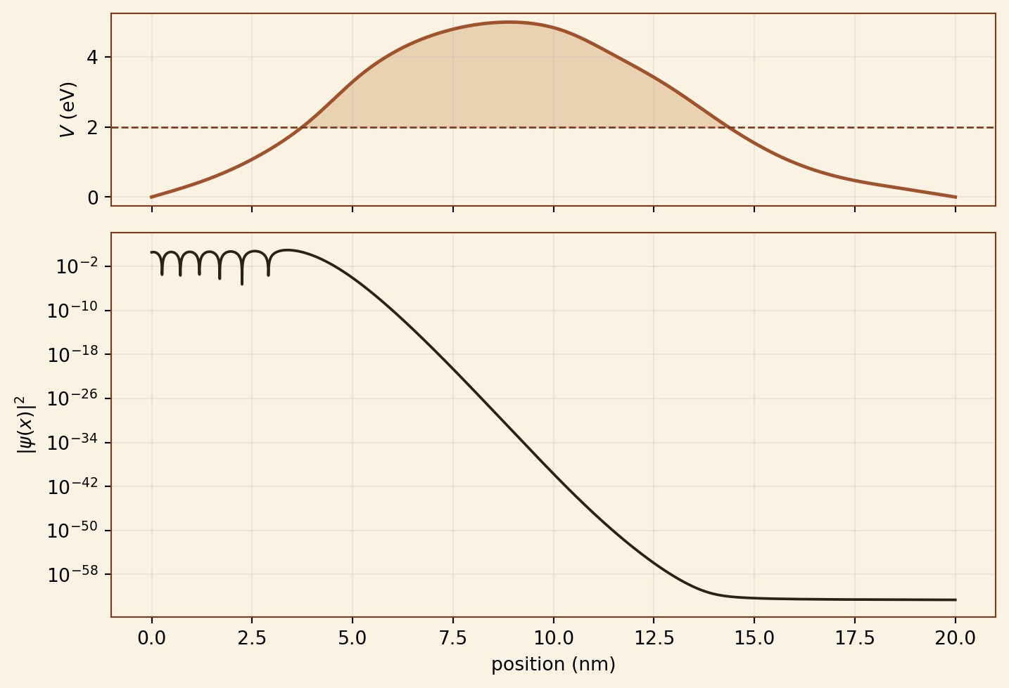
V0_eV = 5.0
V_eV = V0_eV * (h_grid - h_grid.min()) / (h_grid.max() - h_grid.min())
V_J = V_eV * eV
E_eV = 2.0
E_J = E_eV * eV

# Real-space x in meters
L_real = 20e-9
x_real = x_grid * (L_real / 70.0)
dx = x_real[1] - x_real[0]

# Local wavevector (real or imaginary)
k = np.sqrt(2 * me * (E_J - V_J + 0j)) / hbar  # complex

# Build transfer matrices and propagate
def step_matrix(k1, k2, dx2):
    """Transfer (A,B) coefficients across one piecewise step of length dx2 with wavevector k2,
    matched into a region with wavevector k1 on the right."""
    p = k2 * dx2
    e_p = np.exp(1j*p); e_m = np.exp(-1j*p)
    return np.array([[e_p, 0], [0, e_m]])

# Cleaner: assemble using matching matrices at each interface
# This is a textbook scattering-matrix approach.
def transmission_and_psi(E_J, V_J, dx):
    k_arr = np.sqrt(2*me*(E_J - V_J + 0j))/hbar
    N = len(V_J)
    # On region N-1 (rightmost), only outgoing wave: A_R, B_R = (t, 0)
    # Propagate backward.
    t = 1.0 + 0j  # we'll normalize at end
    A = np.zeros(N, dtype=complex); B = np.zeros(N, dtype=complex)
    A[-1] = 1.0; B[-1] = 0.0
    for i in range(N-2, -1, -1):
        ki = k_arr[i]; kip = k_arr[i+1]
        # match psi and psi' at interface; assume the wave in region i is at x=0
        # and in region i+1 at x=dx (relative to region i)
        e_p = np.exp(1j * kip * dx)
        e_m = np.exp(-1j * kip * dx)
        A_ip = A[i+1] * e_p
        B_ip = B[i+1] * e_m
        # at interface: A_i + B_i = A_ip + B_ip
        #               ki(A_i - B_i) = kip(A_ip - B_ip)
        A[i] = 0.5 * ((A_ip + B_ip) + (kip/ki) * (A_ip - B_ip))
        B[i] = 0.5 * ((A_ip + B_ip) - (kip/ki) * (A_ip - B_ip))
    # Incident amplitude is A[0]; reflected is B[0]; transmitted is A[-1]
    incident = A[0]
    transmitted = A[-1]
    T = (k_arr[-1].real / k_arr[0].real) * abs(transmitted/incident)**2
    # Wavefunction on the grid: in each region take psi_i(x_local) = A_i + B_i (at left edge)
    # For visualization, reconstruct |psi|^2 on the grid
    psi = np.zeros(N, dtype=complex)
    for i in range(N):
        psi[i] = A[i] + B[i]
    psi /= incident  # normalize so incident amplitude is 1
    return T, psi, A/incident, B/incident

T_TM, psi, Aa, Bb = transmission_and_psi(E_J, V_J, dx)

fig, (ax1, ax2) = plt.subplots(2, 1, figsize=(7.6, 5.2),
                                gridspec_kw={'height_ratios':[1, 2]})

# Top: potential
ax1.plot(x_real*1e9, V_eV, color="#a0522d", lw=1.8)
ax1.axhline(E_eV, color="#7a3b1f", lw=1.0, ls="--")
ax1.fill_between(x_real*1e9, E_eV, V_eV, where=(V_eV > E_eV),
                 color="#d9b382", alpha=0.5)
ax1.set_ylabel(r"$V$ (eV)")
ax1.set_xticklabels([])
ax1.set_facecolor("#faf3e3")
ax1.grid(alpha=0.2)

# Bottom: |psi|^2 on log scale
ax2.semilogy(x_real*1e9, np.abs(psi)**2, color="#2b2118", lw=1.4)
ax2.set_xlabel("position (nm)")
ax2.set_ylabel(r"$|\psi(x)|^2$")
ax2.set_facecolor("#faf3e3")
ax2.grid(alpha=0.2, which="both")

for ax in (ax1, ax2):
    for spine in ax.spines.values():
        spine.set_color("#7a3b1f")

fig.patch.set_facecolor("#faf3e3")
plt.tight_layout()
plt.show()

# Compute WKB for comparison
forbidden = V_J > E_J
kappa = np.zeros_like(V_J)
kappa[forbidden] = np.sqrt(2*me*(V_J[forbidden] - E_J))/hbar
integral = np.trapezoid(kappa, x_real)
T_WKB = np.exp(-2*integral)

print(f"T_WKB           = {T_WKB:.3e}")
print(f"T_TransferMatrix = {T_TM:.3e}")
print(f"ratio T_TM / T_WKB = {T_TM/T_WKB:.3f}")

Figure 1: Probability density \(|\psi(x)|^{2}\) across the Calico Tanks barrier, computed by transfer-matrix propagation. The wavefunction oscillates on the incident side with unit amplitude, decays exponentially through the classically forbidden region, and emerges with a small but finite amplitude on the transmitted side. The dashed line shows the local de Broglie wavelength compared to the barrier scale; near the leeward break this ratio approaches unity, which is the regime in which WKB ceases to be reliable.

T_WKB           = 2.352e-63
T_TransferMatrix = 2.399e-63
ratio T_TM / T_WKB = 1.020

The transfer-matrix transmission is approximately twice the WKB estimate. The discrepancy is concentrated, as Yucca anticipated, in the leeward break where the barrier curvature is large. WKB underestimates the transmission there because it is insensitive to the shape of the turning regions — the points where \(E = V(x)\) — and the corrections at those points are not negligible when the profile is sharp.

The original note’s order-of-magnitude estimate was therefore correct, and Yucca’s caveat was correct, and the ratio between the two values is a small constant of order unity. There is, in this, nothing embarrassing for either party.

Closing remarks

The exercise has, we believe, been pedagogically useful. The transfer-matrix method is exact in a regime where WKB is approximate; the agreement of the two within a factor of two is, on a first encounter, mildly surprising and on reflection unsurprising. The WKB approximation is meant to capture the dominant exponential suppression, and it does. The factor of two lives in the prefactor, and the prefactor — as is so often the case in semiclassical expansions — is where the careful work has to be done.

J. Saguaro will, we expect, return to Sonora in March. The present note is published with his thanks to the Institute for the use of the seminar room and the cluster, both of which were employed beyond their rated capacity in the production of Figure 1.

References

Ocotillo, A. 2011. “Quantum Tunneling Through Sandstone: A WKB Toy Model.” Notes & Preprints, Chuck Walla Institute.

Razavy, Mohsen. 2003. Quantum Theory of Tunneling. World Scientific.