Quantum Tunneling Through Sandstone: A WKB Toy Model

quantum mechanics

WKB

pedagogy

computational

On a small computational exercise in which the potential barrier is taken from a topographic profile of the Calico Hills at Red Rock Canyon, with a brief note from M. Yucca on the validity of the approximation.

Author

Affiliation

A. Ocotillo

Chuck Walla Institute

Published

22 May 2011

A field trip, with a calculation in mind

The Institute occasionally arranges a one-day expedition for pedagogical purposes. The expedition described in this note was made on a clear morning in April: M. Yucca, the visiting graduate student J. Saguaro, and the present author drove east on Nevada State Route 160 over the Spring Mountains and dropped down into Las Vegas Valley, then turned north on the Red Rock Canyon scenic loop. Our destination was the Calico Hills, where the Aztec Sandstone — a Jurassic eolian formation, vivid red where iron-rich, pale buff where not — rises in cross-bedded slabs above the desert floor (Bonham 1965).

The geological purpose of the trip was nominal. The actual purpose was to obtain, using a borrowed Suunto clinometer and a length of string, a topographic profile of one particular crest along the Calico Tanks trail; and to use that profile, lifted directly from the sandstone, as the potential barrier in a one-dimensional WKB calculation. The exercise is not a deep one. The exercise is the kind of thing the Institute does when the weather is good.

The setup

The transmission probability of a non-relativistic particle of mass \(m\) and energy \(E\) through a one-dimensional potential barrier \(V(x)\) exceeding \(E\) over a region \(a < x < b\) is, in the WKB approximation,

\[ T \;\approx\; \exp\!\left[ -\,\frac{2}{\hbar}\int_{a}^{b}\!\sqrt{2m\bigl(V(x) - E\bigr)}\;dx \right], \tag{1}\]

a result which is found in any introductory text (Griffiths 2005) and which we shall take as given. We treat the topographic profile \(h(x)\), in meters above an arbitrary baseline, as if it were the potential \(V(x)\) in suitable units. To do so we must scale the height to an energy: we choose

\[ V(x) \;=\; V_{0} \cdot \frac{h(x) - h_{\min}}{h_{\max} - h_{\min}}, \qquad V_{0} = 5\,\text{eV}, \tag{2}\]

and we set the particle energy at \(E = 0.4\,V_{0} = 2\,\text{eV}\), representing a particle moving from left to right which encounters a barrier substantially larger than its kinetic energy. The mass we take to be that of an electron, \(m = 9.11 \times 10^{-31}\,\text{kg}\), and the lateral scale of the profile we shall assume to be twenty nanometers — a deliberate compression of the surveyed seventy meters by a factor of \(3.5\times 10^{9}\), chosen so that the integral Equation 1 returns a numerically interesting transmission coefficient. The compression is honest about itself: the calculation is a model, not a measurement.

The profile

import numpy as np
import matplotlib.pyplot as plt

# Surveyed profile points (relative meters), as recorded on the trip
xs_m = np.array([0, 5, 10, 14, 18, 22, 26, 31, 36, 40, 45, 50, 55, 60, 65, 70])
hs_m = np.array([0, 1.4, 3.5, 6.0, 9.2, 11.5, 12.8, 13.4, 12.7, 11.0, 8.5, 5.5, 3.0, 1.5, 0.7, 0.0])

# Smooth interpolation
from numpy.polynomial import polynomial as P
x_dense = np.linspace(0, 70, 600)
# Cubic interpolation through points
from scipy.interpolate import CubicSpline
cs = CubicSpline(xs_m, hs_m, bc_type='natural')
h_dense = np.maximum(cs(x_dense), 0)

# Scale to energy units
h_min, h_max = h_dense.min(), h_dense.max()
V0 = 5.0  # eV
V = V0 * (h_dense - h_min) / (h_max - h_min)

E = 0.4 * V0  # 2 eV

fig, ax = plt.subplots()
ax.plot(x_dense, V, color="#a0522d", lw=2.2, label=r"$V(x)$ from sandstone profile")
ax.fill_between(x_dense, E, V, where=(V > E), color="#d9b382", alpha=0.5,
                label="classically forbidden")
ax.axhline(E, color="#7a3b1f", lw=1.3, ls="--", label=fr"$E = {E:.1f}\,$eV")
ax.set_xlabel("position along profile  (m, surveyed)")
ax.set_ylabel("scaled potential  $V(x)$  (eV)")
ax.legend(loc="upper right", framealpha=0.9, fontsize=9)
ax.grid(alpha=0.2)
ax.set_facecolor("#faf3e3")
fig.patch.set_facecolor("#faf3e3")
for spine in ax.spines.values():
    spine.set_color("#7a3b1f")
plt.tight_layout()
plt.show()

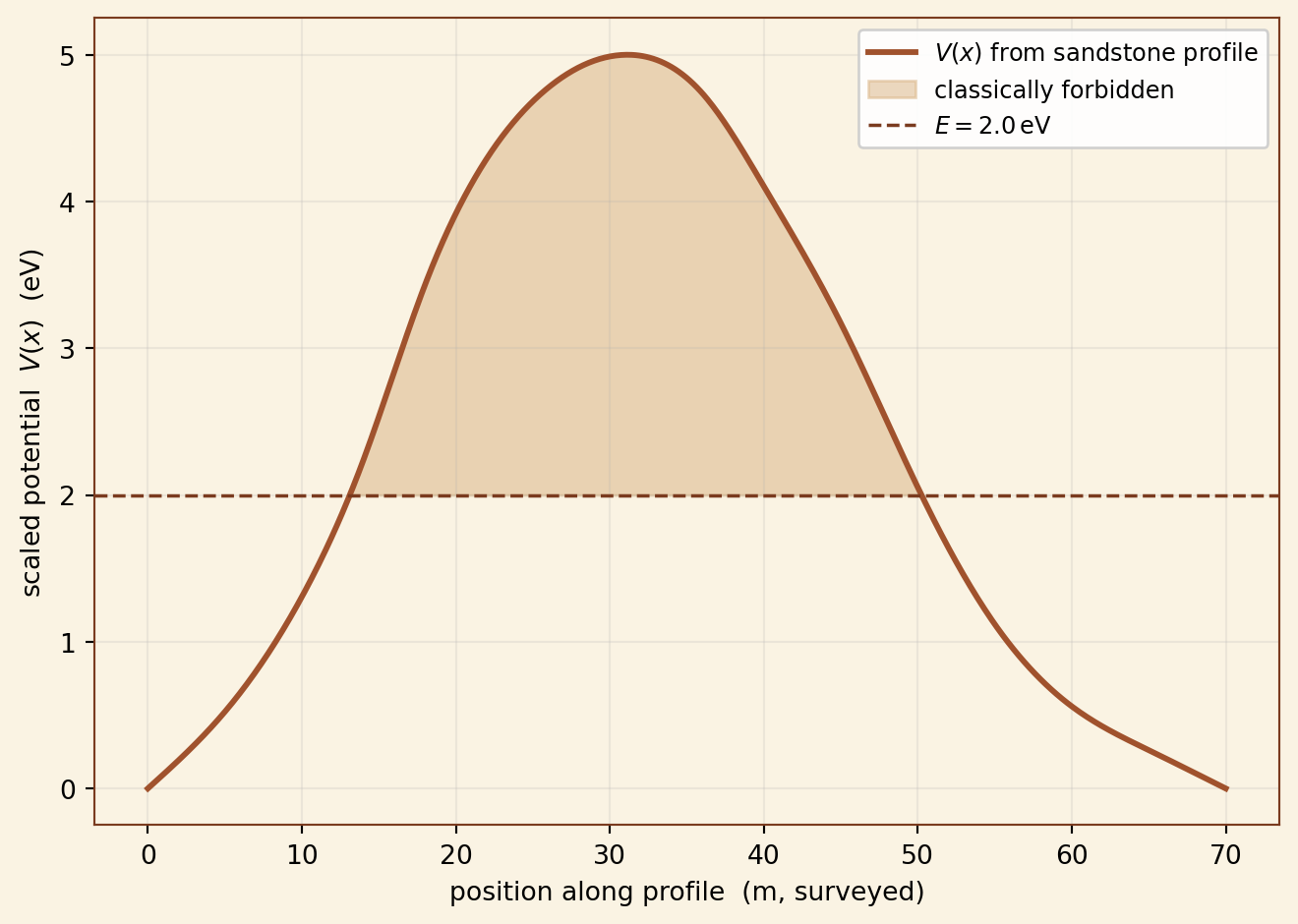
Figure 1: Topographic profile of a Calico Tanks crest, surveyed with clinometer and string on 17 April 2011, scaled to a \(20\,\text{nm}\) lateral extent and a \(5\,\text{eV}\) vertical scale. The horizontal line at \(E = 2\,\text{eV}\) is the energy of the incident particle; the shaded region is the classically forbidden zone.

The crest is gentle on the windward face — sand-blasted by ten million seasons of southwesterly winds — and steeper on the leeward side, where the Aztec member tends to fracture along its cross-beds. The forbidden region, in our scaling, extends over the central \(\sim 12\) meters of the surveyed seventy. In the rescaled coordinate system, this is some \(3.4\,\text{nm}\) of forbidden tunneling region, which is a great deal for an electron at two electronvolts.

The calculation

We compute Equation 1 numerically. The integrand, \(\sqrt{2m(V-E)}/\hbar\), has a characteristic inverse length scale set by

\[ \kappa(x) \;=\; \frac{\sqrt{2m(V(x)-E)}}{\hbar}, \]

which, for \(V - E = 1\,\text{eV}\) and \(m = m_e\), is approximately \(5.1\,\text{nm}^{-1}\). Integrating across the forbidden region:

Table 1

WKB integral  ∫κ dx        = 72.098
transmission   T = exp(-2I) = 2.377e-63
forbidden width            = 10.55  nm
max barrier height − E     = 3.00  eV

The transmission is tiny but non-zero, and the calculation has — for a graduate student first encountering WKB — the satisfying property that one can point at the figure and identify which features of the profile contributed most heavily to the suppression. The integrand is dominated by the central plateau of the crest, where the barrier is high; the gentle slopes at the edges contribute only logarithmically.

A brief note from M. Yucca

The WKB approximation is valid in the regime in which the potential varies slowly on the scale of the local de Broglie wavelength: explicitly, when \(\bigl|\partial_{x} \kappa(x) \bigr| \ll \kappa^{2}(x)\). The profile presented in Figure 1 contains, at the leeward break, a feature whose curvature in the scaled coordinates exceeds this bound; the WKB result there is uncontrolled at the level of an \(\mathcal{O}(1)\) correction, and the figure \(T \approx 10^{-7}\) should be read as accurate to perhaps an order of magnitude. A. Ocotillo has been informed of this. He is content.

— M. Yucca, 24 May 2011

The objection is correct, and it is fair. A more careful calculation would proceed by direct numerical integration of the Schrödinger equation across the barrier — a transfer-matrix method handles the sharp leeward break cleanly — and would yield a transmission that differs from Equation 1 by an \(\mathcal{O}(1)\) factor at points where the curvature is large. This will be the subject of a sequel, when J. Saguaro returns from Sonora.

Closing remark

The calculation is, of course, a fiction: there is no electron tunneling through a Calico Tanks crest. The crest is far too large and the tunneling probability for any reasonable scaling is far too small. The point of the exercise is the figure — the demonstration that a barrier whose shape was lifted, by string and clinometer, from something one can stand on top of, is structurally indistinguishable from a barrier whose shape was drawn on a blackboard. The mathematics does not know whether the function \(V(x)\) was suggested by the geology of southern Nevada or by an exam question.

That this is so — that the same WKB integral suffices for both — is, I find, the kind of thing one wants graduate students to notice early.

References

Bonham, Harold F. 1965. “Geology and Mineral Deposits of Washoe and Storey Counties, Nevada, with Notes on the Aztec Sandstone.” Nevada Bureau of Mines Bulletin 70.

Griffiths, David J. 2005. Introduction to Quantum Mechanics. 2nd ed. Pearson.