where \(a\) is the proper acceleration. Equation Equation 1, due to Unruh (1976) (with antecedents in Fulling (1973) and Davies (1975)), is a statement about how the Minkowski vacuum decomposes when one uses Rindler coordinates rather than inertial ones: the same state which an inertial observer calls empty is, for the accelerating observer, a mixed state at temperature \(T_{\text{U}}\).
The derivation involves the Bogoliubov coefficients between Minkowski and Rindler mode expansions, and we will not reproduce it here; the account in Birrell and Davies (1982) is canonical and good. The present note concerns the magnitude of the effect, with particular reference to acceleration scales that may be encountered in the operation of the Institute’s vehicle.
Numerical scale
Substituting fundamental constants into Equation 1, the prefactor is
In other words, an acceleration of \(1\,\text{m/s}^{2}\) corresponds to a Unruh temperature of approximately \(4 \times 10^{-21}\,\text{K}\). To produce a thermal bath of \(1\,\text{K}\), one requires
which is some nineteen orders of magnitude larger than the surface gravity of the Earth. The Unruh effect is, by any standard, small.
The pickup truck
The Institute maintains a 1986 Chevrolet K10, in which the Director’s weekly supply run to Pahrump is conducted. Empirical determination, made on the long straight section of Nevada State Route 160 east of the Last Chance Road junction, places the vehicle’s acceleration from rest to \(60\,\text{mph}\) at approximately ten seconds, corresponding to
This is approximately \(10^{-19}\) times the temperature of the cosmic microwave background, \(10^{-22}\) times the temperature at which oxygen liquefies, and \(10^{-29}\) times the cabin temperature in August. The driver does not, on these grounds, feel notably warmer when she depresses the accelerator.
A landscape of accelerations
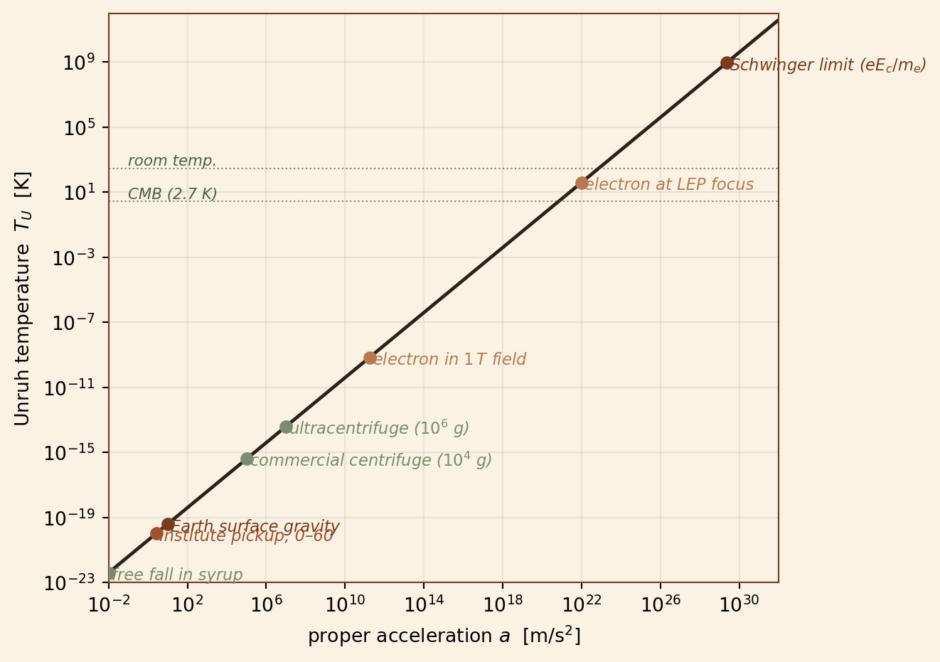
The plot below places the truck on a logarithmic landscape of accelerations of physical interest, with the corresponding Unruh temperature on the right axis.
import numpy as npimport matplotlib.pyplot as plta = np.logspace(-2, 32, 500) # m/s^2T =4.06e-21* a # Kevents = [ ("free fall in syrup", 1e-2, "#7a8b6f"), ("Institute pickup, 0–60", 2.7, "#a0522d"), ("Earth surface gravity", 9.81, "#7a3b1f"), ("commercial centrifuge ($10^4$ g)", 1e5, "#7a8b6f"), ("ultracentrifuge ($10^6$ g)", 1e7, "#7a8b6f"), ("electron in $1\\,$T field", 1.76e11,"#b8794f"), ("electron at LEP focus", 1e22, "#b8794f"), ("Schwinger limit ($eE_c/m_e$)",2.3e29, "#7a3b1f"),]fig, ax = plt.subplots()ax.loglog(a, T, color="#2b2118", lw=1.8)for label, a_val, color in events: T_val =4.06e-21* a_val ax.plot(a_val, T_val, "o", color=color, markersize=6, zorder=5) ax.annotate(label, xy=(a_val, T_val), xytext=(a_val*1.4, T_val*0.35), fontsize=8.5, color=color, fontstyle="italic")# Reference horizontalsfor T_ref, name, color in [(2.7, "CMB (2.7 K)", "#4f5e48"), (300, "room temp.", "#4f5e48")]: ax.axhline(T_ref, color=color, lw=0.8, ls=":", alpha=0.7) ax.text(1e-1, T_ref*1.5, name, fontsize=8, color=color, fontstyle="italic")ax.set_xlabel(r"proper acceleration $a$[m/s$^2$]")ax.set_ylabel(r"Unruh temperature $T_U$[K]")ax.set_xlim(1e-2, 1e32)ax.set_ylim(1e-23, 1e12)ax.grid(alpha=0.25, which="both")ax.set_facecolor("#faf3e3")fig.patch.set_facecolor("#faf3e3")for spine in ax.spines.values(): spine.set_color("#7a3b1f")plt.tight_layout()plt.show()
Figure 1: Unruh temperatures across nineteen orders of magnitude. The Institute’s pickup, surface gravity, and a fast centrifuge are far below the temperatures attainable by particles in strong fields.
Three observations.
First: nothing one can do with macroscopic objects produces a Unruh temperature within sixteen orders of magnitude of the CMB. Detection in a laboratory is, accordingly, hard.
Second: the right-hand end of the plot — accelerations near the Schwinger critical field, \(E_{c} \approx 1.3 \times 10^{18}\,\text{V/m}\) — begins to produce Unruh temperatures comparable to the rest mass of the electron. Here the linear approximation Equation 1 becomes inadequate and one must consider full pair production (Schwinger 1951). This is the regime of next-generation laser facilities and certain astrophysical environments; it is not the regime of the highway.
Third: the existence of Equation 1, even at unmeasurable scales, is a statement about the vacuum — namely, that what counts as the vacuum depends on the observer’s worldline. This is the same observation that, extrapolated to a black hole horizon, gives Hawking radiation (Hawking 1975), and the parallel is not coincidental: a free-falling observer near a Schwarzschild horizon is the local analogue of a uniformly accelerating observer in flat spacetime.
Closing remarks
The Unruh effect is, in our pedagogical experience, the cleanest illustration available of the proposition that the vacuum is a frame of reference. Whether the effect has been definitively observed is a question on which the Institute does not take a position; the proposed detection schemes (Bell and Leinaas 1987; Rogers 1988) involve very high accelerations of polarized electrons in storage rings, and the interpretation of the data is contested. We watch with patience.
It remains, in any case, a useful disciplinary fact that one cannot warm one’s dinner by driving fast.
References
Bell, J. S., and J. M. Leinaas. 1987. “The Unruh Effect and Quantum Fluctuations of Electrons in Storage Rings.”Nucl. Phys. B 284: 488–508.
Birrell, N. D., and P. C. W. Davies. 1982. Quantum Fields in Curved Space. Cambridge University Press.
Davies, P. C. W. 1975. “Scalar Production in Schwarzschild and Rindler Metrics.”J. Phys. A 8: 609–16.
Fulling, S. A. 1973. “Nonuniqueness of Canonical Field Quantization in Riemannian Space-Time.”Phys. Rev. D 7: 2850–62.
Hawking, S. W. 1975. “Particle Creation by Black Holes.”Commun. Math. Phys. 43: 199–220.
Rogers, J. 1988. “Detector for the Acceleration-Induced Vacuum Excitation.”Phys. Rev. Lett. 61: 2113–16.